
To solve the diffusion equation, which is a second-order partial differential equation throughout the reactor volume, it is necessary to specify certain boundary conditions.
In previous chapters, we introduced two bases for the derivation of the diffusion equation:
![]()
which states that neutrons diffuse from high concentration (high flux) to low concentration.
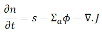
which states that rate of change of neutron density = production rate – absorption rate – leakage rate.
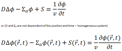
We return now to the neutron balance equation and substitute the neutron current density vector by J = -D∇Ф. Assuming that ∇.∇ = ∇2 = Δ (therefore div J = -D div (∇Ф) = -DΔФ) we obtain the diffusion equation.
See also: Diffusion Coefficient
See also: Neutron Cross-section
See also: Neutron Flux Density
The derivation of the diffusion equation is based on Fick’s law which is derived under many assumptions. Therefore, the diffusion equation cannot be exact or valid at places with strongly differing diffusion coefficients or in strongly absorbing media. This implies that the diffusion theory may show deviations from a more accurate solution of the transport equation in the proximity of external neutron sinks, sources, and media interfaces.
Physical Interpretation of Fick’s Law
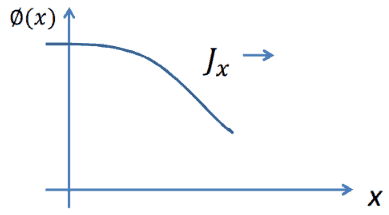 The physical interpretation is similar to the fluxes of gases. The neutrons exhibit a net flow in the direction of least density. This is a natural consequence of greater collision densities at positions of greater neutron densities.
Consider neutrons passing through the plane at x=0 from left to right due to collisions to the plane’s left. Since the concentration of neutrons and the flux is larger for negative values of x, there are more collisions per cubic centimeter on the left. Therefore more neutrons are scattered from left to right, then the other way around. Thus the neutrons naturally diffuse toward the right.
Boundary Conditions
To solve the diffusion equation, which is a second-order partial differential equation throughout the reactor volume, it is necessary to specify certain boundary conditions. It is very dependent on the complexity of certain problem. One-dimensional problems solutions of diffusion equation contain two arbitrary constants. Therefore, in order to solve one-dimensional one-group diffusion equation, we need two boundary conditions to determine these coefficients. The most convenient boundary conditions are summarized in following few points:
The diffusion equation is mostly solved in media with high densities, such as neutron moderators (H2O, D2O, or graphite). The problem is usually bounded by air. The mean free path of a neutron in the air is much larger than in the moderator so that it is possible to treat it as a vacuum in neutron flux distribution calculations. The vacuum boundary condition supposes that no neutrons are entering a surface.
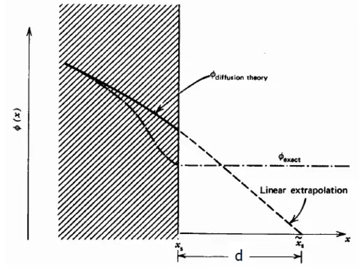
If we consider that no neutrons are reflected from the vacuum back to the volume, the following condition can be derived from Fick’s law:
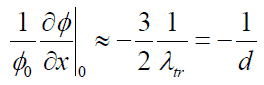
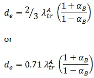
Where d ≈ ⅔ λtr is known as the extrapolated length, for homogeneous, weakly absorbing media, an exact solution of the mono-energetic transport equation in this case yields d ≈ 0.7104 λtr. The geometric interpretation of the previous equation is that the relative neutron flux near the boundary has a slope of -1/d, i.e., the flux would extrapolate linearly to 0 at a distance d beyond the boundary. This zero flux boundary condition is more straightforward and can be written mathematically as:

If d is not negligible, physical dimensions of the reactor are increased by d, and extrapolated boundary is formulated with dimension Re = R + d, and this condition can be written as Φ(R + d) = Φ(Re) = 0.
It may seem the flux goes to 0 at an extrapolated length beyond the boundary. This interpretation is not correct. The flux cannot go to zero in a vacuum because there are no absorbers to absorb the neutrons. The flux only appears to be heading to the zero value at the extrapolation point.
Note that the equation d ≈ 0.7104 λtr is applicable to plane boundaries only. The formulas for curved boundaries can differ slightly. However, the difference is small unless the radius of curvature of the boundary is of the same order of magnitude as the extrapolated length.
Typical values of the extrapolated length:
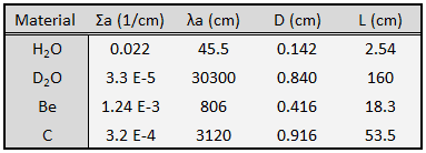
The most common moderators have following diffusion coefficients (for thermal neutrons):
D(H2O) = 0.142 cm
D(D2O) = 0.84 cm
D(Be) = 0.416 cm
D(C) = 0.916 cm
The thermal neutron extrapolated lengths are given by:
d ≈ 0.7104 λtr = 0.7104 x 3 x D
therefore:
H2O: d ≈ 0.30 cm
D2O: d ≈ 1.79 cm
Be: d ≈ 0.88 cm
C: d ≈ 1.95 cm
As can be seen, this approximation is valid when the dimension L of the diffusing medium is much larger than the extrapolated length, L >> d.
![]()
These conditions are often used to eliminate unnecessary functions from solutions.
It must be added, as J must be continuous, the flux gradient will show a jump if the diffusion coefficients in both media differ from each other.
On this special interface, we shall apply an albedo boundary condition to represent the neutron reflector. Albedo, the latin word for “whiteness”, was defined by Lambert as the fraction of the incident light reflected diffusely by a surface.
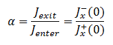
In reactor engineering, albedo, or the reflection coefficient, is defined as the ratio of exiting to entering neutrons, and we can express it in terms of neutron currents as:
For sufficiently thick reflectors, it can be derived that albedo becomes

where Drefl is the diffusion coefficient in the reflector and the Lrefl is the diffusion length in the reflector.
If we are not interested in the neutron flux distribution in the reflector (let say in the slab B) but only in the effect of the reflector on the neutron flux distribution in the medium (let say in slab A), the albedo of the reflector can be used as a boundary condition for the diffusion equation solution. This boundary condition is similar to the vacuum boundary condition, i.e., Φ(Ralbedo) = 0, where Ralbedo = R + de and
Solutions of the Diffusion Equation – Non-multiplying Systems
As was previously discussed, the diffusion theory is widely used in the core design of the current Pressurized Water Reactors (PWRs) or Boiling Water Reactors (BWRs). This section is not about such calculations but provides illustrative insights, how can be the neutron flux distributed in any diffusion medium. In this section, we will solve diffusion equations:
in various geometries that satisfy the boundary conditions discussed in the previous section.
We will start with simple systems and increase complexity gradually. The most important assumption is that all neutrons are lumped into a single energy group. They are emitted and diffuse at thermal energy (0.025 eV).
In the first section, we will deal with neutron diffusion in a non-multiplying system, i.e., in the system where fissile isotopes are missing, the fission cross-section is zero. An external neutron source emits the neutrons. We will assume that the system is uniform outside the source, i.e., D and Σa are constants.
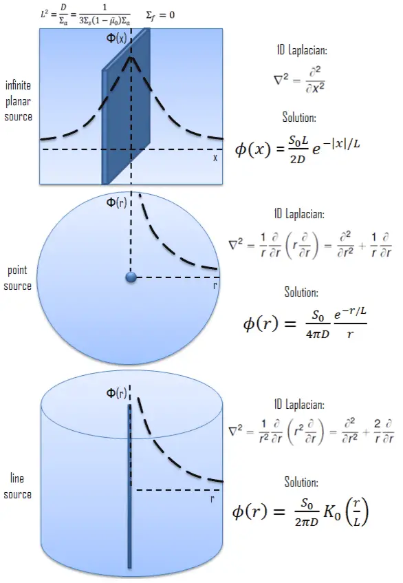
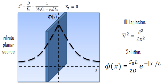 Let assume the neutron source (with strength S0) as an infinite plane source (in y-z plane geometry). In this geometry, the flux varies slowly in y and z allowing us to eliminate the y and z derivatives from ∇2. The flux is then a function of x only, and therefore the Laplacian and diffusion equation (outside the source) can be written as (everywhere except x = 0):

For x > 0, this diffusion equation has two possible solutions exp(x/L) and exp(-x/L), which give a general solution:
Φ(x) = Aexp(x/L) + Cexp(-x/L)
Note that B is not usually used as a constant because B is reserved for a buckling parameter. To determine the coefficients A and C, we must apply boundary conditions.
From finite flux condition (0≤ Φ(x) < ∞), which required only reasonable values for the flux, it can be derived that A must be equal to zero. The term exp(x/L) goes to ∞ as x ➝∞ and therefore cannot be part of a physically acceptable solution for x > 0. The physically acceptable solution for x > 0 must then be:
Φ(x) = Ce-x/L
where C is a constant that can be determined from the source condition at x ➝0.
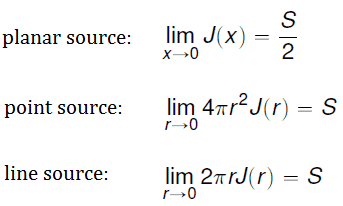
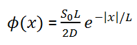
If S0 is the plane’s source strength per unit area, then the number of neutrons crossing outwards per unit area in the positive x-direction must tend to S0 /2 as x ➝0.

So that the solution may be written:
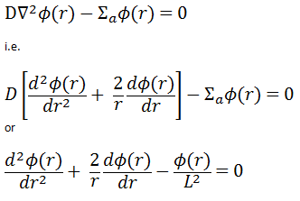
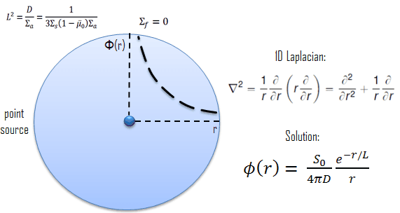 Let assume the neutron source (with strength S0) as an isotropic point source situated in spherical geometry. This point source is placed at the origin of coordinates. To solve the diffusion equation, we have to replace the Laplacian with its spherical form:

We can replace the 3D Laplacian with its one-dimensional spherical form because there is no dependence on the angle (whether polar or azimuthal). The source is assumed to be an isotropic source (there is the spherical symmetry). The flux is then a function of radius – r only, and therefore the diffusion equation (outside the source) can be written as (everywhere except r = 0):
If we make the substitution Φ(r) = 1/r ψ(r), the equation simplifies to:
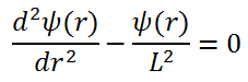
For r > 0, this differential equation has two possible solutions exp(r/L) and exp(-r/L), which give a general solution:
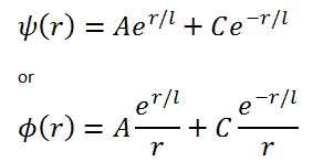
Note that B is not usually used as a constant because B is reserved for a buckling parameter. To determine the coefficients A and C, we must apply boundary conditions.
To find constants A and C, we use the identical procedure as in the case of the infinite planar source. From finite flux condition (0≤ Φ(r) < ∞), which required only reasonable values for the flux, it can be derived that A must be equal to zero. The term exp(r/L)/r goes to ∞ as r ➝∞ and therefore cannot be part of a physically acceptable solution for r > 0. The physically acceptable solution for r > 0 must then be:
Φ(r) = Ce-r/L/r
where C is a constant that can be determined from source condition at x ➝0.
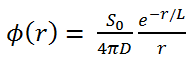
If S0 is the source strength, then the number of neutrons crossing a sphere outwards in the positive r-direction must tend to S0 as r ➝0.
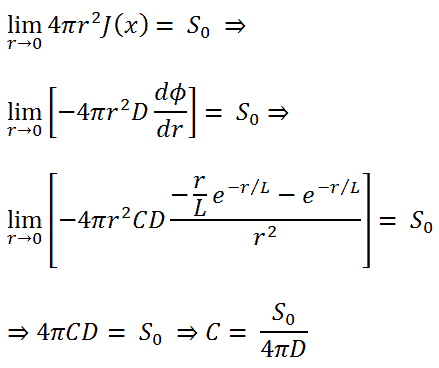
So that the solution may be written:
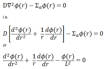
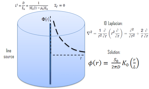 Let assume the neutron source (with strength S0) as an isotropic line source situated in an infinite cylindrical geometry. This line source is placed at r = 0. To solve the diffusion equation, we have to replace the Laplacian by its cylindrical form:
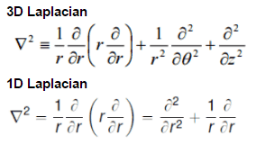
Since there is no dependence on angle Θ and z-coordinate, we can replace the 3D Laplacian with its one-dimensional form, and we can solve the problem only in the radial direction. The source is assumed to be an isotropic source. Since the flux is a function of radius – r only, the diffusion equation (outside the source) can be written as (everywhere except r = 0):
 This differential equation is called Bessel’s equation, and it is well known to mathematicians. In this case, the solutions to the Bessel’s equation are called the modified Bessel functions (or occasionally the hyperbolic Bessel functions) of the first and second kind, Iα(x) and Kα(x), respectively.
For r > 0, this differential equation has two possible solutions, I0(r/L) and K0(r/L), the modified Bessel functions of order zero, which give a general solution:

To find constants A and C, we use the identical procedure as in the case of the infinite planar source. From finite flux condition (0≤ Φ(r) < ∞), which required only reasonable values for the flux, it can be derived that A must be equal to zero. The term I0(r/L) goes to ∞ as r ➝∞ and therefore cannot be part of a physically acceptable solution for r > 0. The physically acceptable solution for r > 0 must then be:
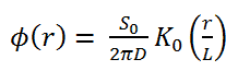
Φ(r) = C.K0(r/L)
where C is a constant that can be determined from the source condition at r ➝0.
If S0 is the source strength, then the number of neutrons crossing a cylinder outwards in the positive r-direction must tend to S0 as r ➝0.
So that the solution may be written:
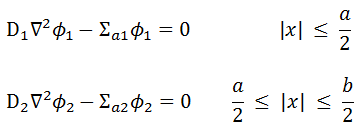
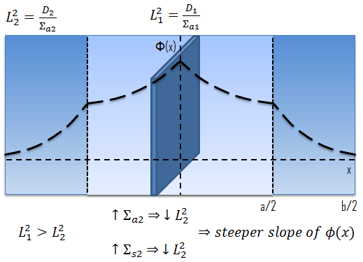
where a is the real width of zone 1 and b is the outer dimension of the diffusion environment, including the extrapolated distance. With problems involving two different diffusion media, the interface boundary conditions play a crucial role and must be satisfied:
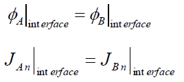
At interfaces between two different diffusion media (such as between the reactor core and the neutron reflector), on physical grounds, the neutron flux and the normal component of the neutron current must be continuous. In other words, φ and J are not allowed to show a jump.
1., 2. Interface Conditions
It must be added, as J must be continuous, the flux gradient will show a jump if the diffusion coefficients in both media differ from each other. Since the solution of these two diffusion equations requires four boundary conditions, we have to use two boundary conditions more.
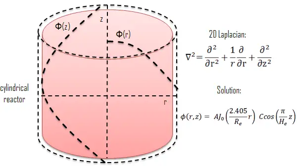
3. Finite Flux Condition
The solution must be finite in those regions where the equation is valid, except perhaps at artificial singular points of a source distribution. This boundary condition can be written mathematically as:
![]() 4. Source Condition
4. Source Condition
The presence of the neutron source can be used as a boundary condition because it is necessary that all neutrons flowing through the bounding area of the source must come from the neutron source. This boundary condition depends on the source geometry, and for planar source can be written mathematically as:
![]()
For x > 0, these diffusion equations have the following appropriate solutions:
Φ1(x) = A1exp(x/L1) + C1exp(-x/L1)
and
Φ2(x) = A2exp(x/L2) + C2exp(-x/L2)
where the four constants must be determined with the use of the four boundary conditions. The typical neutron flux distribution in a simple two-region diffusion problem is shown in the picture below.
Solutions of the Diffusion Equation – Multiplying Systems
In the previous section, it has been considered that the environment is non-multiplying. In a non-multiplying environment, neutrons are emitted by a neutron source situated in the center of the coordinate system and then freely diffuse through media. We are now prepared to consider neutron diffusion in the multiplying system containing fissionable nuclei (i.e., Σf ≠ 0). In this multiplying system, we will also study the spatial distribution of neutrons, but in contrast to the non-multiplying environment, these neutrons can trigger nuclear fission reactions.
The required condition for a stable, self-sustained fission chain reaction in a multiplying system (in a nuclear reactor) is that exactly every fission initiates another fission. The minimum condition is for each nucleus undergoing fission to produce, on average, at least one neutron that causes fission of another nucleus. Also, the number of fissions occurring per unit time (the reaction rate) within the system must be constant.
This condition can be expressed conveniently in terms of the multiplication factor. The infinite multiplication factor is the ratio of the neutrons produced by fission in one neutron generation to the number of neutrons lost through absorption in the preceding neutron generation. This can be mathematically expressed as shown below.
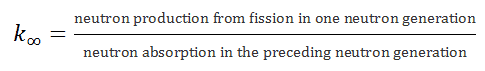
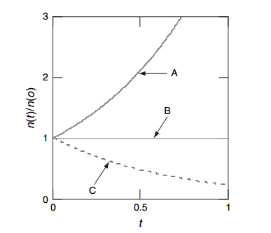
The infinite multiplication factor in a multiplying system measures the change in the fission neutron population from one neutron generation to the subsequent generation.
- k∞ < 1. Suppose the multiplication factor for a multiplying system is less than 1.0. In that case, the number of neutrons decreases in time (with the mean generation time), and the chain reaction will never be self-sustaining. This condition is known as the subcritical state.
- k∞ = 1. If the multiplication factor for a multiplying system is equal to 1.0, then there is no change in neutron population in time, and the chain reaction will be self-sustaining. This condition is known as the critical state.
- k∞ > 1. If the multiplication factor for a multiplying system is greater than 1.0, then the multiplying system produces more neutrons than are needed to be self-sustaining. The number of neutrons is exponentially increasing in time (with the mean generation time). This condition is known as the supercritical state.
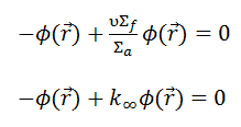
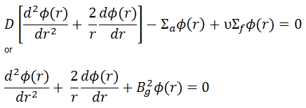
In this section, we will solve the following diffusion equation
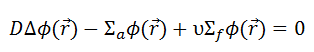
in various geometries that satisfy the boundary conditions. In this equation, ν is the number of neutrons emitted in fission, and Σf is the macroscopic cross-section of the fission reaction. Ф denotes a reaction rate. For example, the fission of 235U by thermal neutron yields 2.43 neutrons.
 It must be noted that we will solve the diffusion equation without any external source. This is very important because such an equation is a linear homogeneous equation in the flux. Therefore if we find one solution of the equation, then any multiple is also a solution. This means that the absolute value of the neutron flux cannot possibly be deduced from the diffusion equation. This is different from problems with external sources, which determine the absolute value of the neutron flux.
We will start with simple systems (planar) and increase complexity gradually. The most important assumption is that all neutrons are lumped into a single energy group. They are emitted and diffuse at thermal energy (0.025 eV). Solutions of diffusion equations, in this case, provide illustrative insights, how can be the neutron flux distributed in a reactor core.
Since the neutron current is equal to zero (J = -D∇Ф, where Ф is constant), the diffusion equation in the infinite uniform multiplying system must be:
![]()
The only solution of this equation is a trivial solution, i.e., Ф = 0, unless Σa = νΣf. This equation (Σa = νΣf) is the critical condition for an infinite reactor and expresses the perfect balance (critical state) between neutron absorption and neutron production. This balance must be continuously maintained to have a steady-state neutron flux.
Infinite Multiplication Factor
In this section, the infinite multiplication factor, k∞, will be defined from another point of view than in section – Nuclear Chain Reaction.
As can be seen, we can rewrite the diffusion equation in the following way, and we can define a new factor – k∞ = νΣf / Σa:
A non-trivial solution of this equation is guaranteed when k∞ = νΣf / Σa = 1. On the other hand, we have no information about the neutron flux in such a critical reactor. The neutron flux can have any value, and the critical uniform infinite reactor can operate at any power level. It should be noted this theory can be used for a reactor at low power levels, hence “zero power criticality”.
In a power reactor core, the power level does not influence the criticality of a reactor unless thermal reactivity feedbacks act (operation of a power reactor without reactivity feedbacks is between 10E-8% – 1% of rated power).
See also: Reactor Criticality
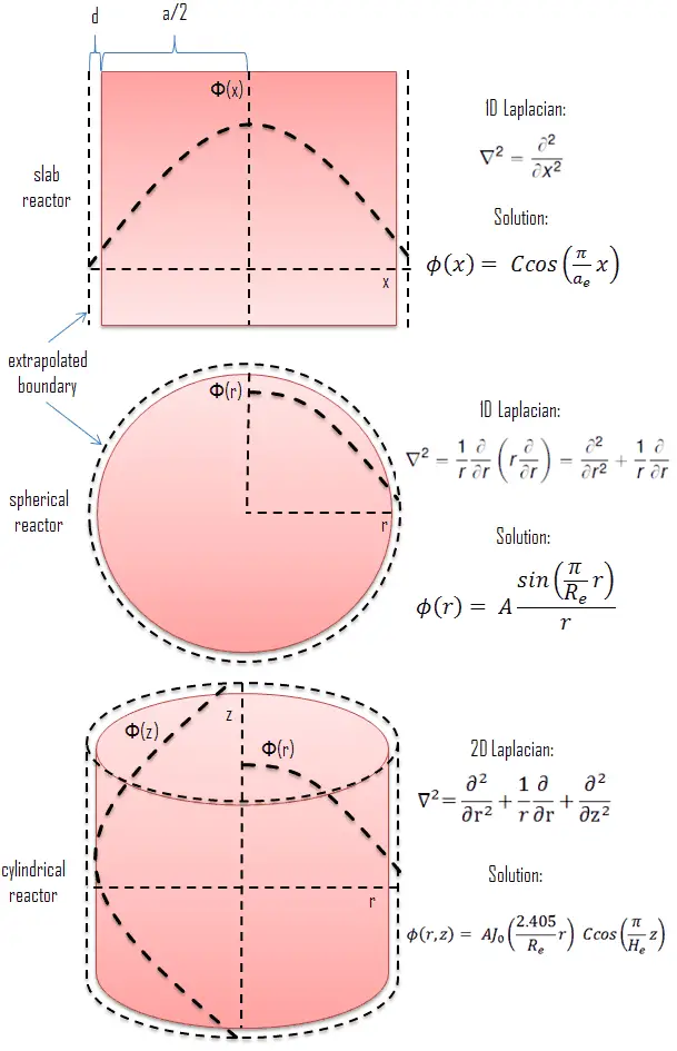
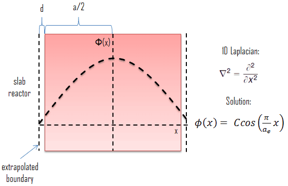 Let assume a uniform reactor (multiplying system) in the shape of a slab of physical width a in the x-direction and infinite in the y- and z-directions. This reactor is situated in the center at x=0. In this geometry, the flux does not vary in y and z allowing us to eliminate the y and z derivatives from ∇2. The flux is then a function of x only, and therefore the Laplacian and diffusion equation can be written as:
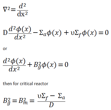
The quantity Bg2 is called the geometrical buckling of the reactor and depends only on the geometry. This term is derived from the notion that the neutron flux distribution is somehow “buckled” in a homogeneous finite reactor. It can be derived the geometrical buckling is the negative relative curvature of the neutron flux (Bg2 = ∇2Ф(x) / Ф(x)). The neutron flux has more concave downward or “buckled” curvature (higher Bg2) in a small reactor than in a large one. This is a very important parameter, and it will be discussed in the following sections.
For x > 0, this diffusion equation has two possible solutions sin(Bgx) and cos(Bgx), which give a general solution:
Φ(x) = A.sin(Bgx) + C.cos(Bg x)
From finite flux condition (0≤ Φ(x) < ∞), which required only reasonable values for the flux, it can be derived that A must be equal to zero. The term sin(Bgx) goes to negative values as x goes to negative values, and therefore it cannot be part of a physically acceptable solution. The physically acceptable solution must then be:
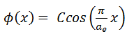
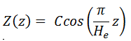
Φ(x) = C.cos(Bg x)
where Bg can be determined from the vacuum boundary condition.
The vacuum boundary condition requires the relative neutron flux near the boundary to have a slope of -1/d, i.e., the flux would extrapolate linearly to 0 at a distance d beyond the boundary. This zero flux boundary condition is more straightforward and can be written mathematically as:

If d is not negligible, physical dimensions of the reactor are increased by d, and an extrapolated boundary is formulated with dimension ae/2 = a/2 + d. This condition can be written as Φ(a/2 + d) = Φ(ae/2) = 0.
Therefore, the solution must be Φ(ae/2) = C.cos(Bg .ae/2) = 0 and the values of geometrical buckling, Bg, are limited to Bg = nπ/a_e, where n is any odd integer. The only one physically acceptable odd integer is n=1 because higher values of n would give cosine functions which would become negative for some values of x. The solution of the diffusion equation is:
It must be added the constant C cannot be obtained from this diffusion equation because this constant gives the absolute value of neutron flux. The neutron flux can have any value, and the critical reactor can operate at any power level. It should be noted the cosine flux shape is only in a hypothetical case in a uniform homogeneous reactor at low power levels (at “zero power criticality”).
In the power reactor core (at full power operation), the neutron flux can reach, for example, about 3.11 x 10¹³ neutrons.cm-2.s-1, but this value depends significantly on many parameters (type of fuel, fuel burnup, fuel enrichment, position in fuel pattern, etc.).
The power level does not influence the criticality (keff) of a power reactor unless thermal reactivity feedbacks act (operation of a power reactor without reactivity feedbacks is between 10E-8% – 1% of rated power).
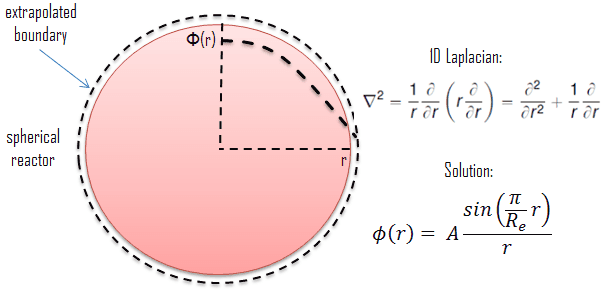 Let us assume a uniform reactor (multiplying system) in the shape of a sphere of physical radius R. The spherical reactor is situated in spherical geometry at the origin of coordinates. To solve the diffusion equation, we have to replace the Laplacian with its spherical form:
We can replace the 3D Laplacian with its one-dimensional spherical form because there is no dependence on an angle (whether polar or azimuthal). The source term is assumed to be isotropic (there is the spherical symmetry). The flux is then a function of radius – r only, and therefore the diffusion equation can be written as:
The solution of the diffusion equation is based on a substitution Φ(r) = 1/r ψ(r), that leads to an equation for ψ(r):
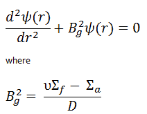
For r > 0, this differential equation has two possible solutions, sin(Bgr) and cos(Bgr), which give a general solution:
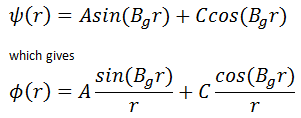
From finite flux condition (0≤ Φ(r) < ∞), which required only reasonable values for the flux, it can be derived that C must be equal to zero. The term cos(Bgr)/r goes to ∞ as r ➝0 and therefore cannot be part of a physically acceptable solution. The physically acceptable solution must then be:
Φ(r) = A sin(Bgr)/r
The vacuum boundary condition requires the relative neutron flux near the boundary to have a slope of -1/d, i.e., the flux would extrapolate linearly to 0 at a distance d beyond the boundary. This zero flux boundary condition is more straightforward and can be written mathematically as:
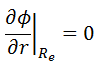
If d is not negligible, physical dimensions of the reactor are increased by d, and extrapolated boundary is formulated with dimension Re = R + d, and this condition can be written as Φ(R + d) = Φ(Re) = 0.
Therefore, the solution must be Φ(Re) = A sin(BgRe)/Re = 0, and the values of geometrical buckling, Bg, are limited to Bg = nπ/Re, where n is any odd integer. The only one physically acceptable odd integer is n=1 because higher values of n would give sine functions which would become negative for some values of x before returning to 0 at Re. The solution of the diffusion equation is:
It must be added the constant A cannot be obtained from this diffusion equation because this constant gives the absolute value of neutron flux. The neutron flux can have any value, and the critical reactor can operate at any power level. It should be noted this flux shape is only in a hypothetical case in a uniform homogeneous spherical reactor at low power levels (at “zero power criticality”).
In a power reactor core, the neutron flux can reach, for example, about 3.11 x 10¹³ neutrons.cm-2.s-1, but this value depends significantly on many parameters (type of fuel, fuel burnup, fuel enrichment, position in fuel pattern, etc.).
The power level does not influence the criticality (keff) of a power reactor unless thermal reactivity feedbacks act (operation of a power reactor without reactivity feedbacks is between 10E-8% – 1% of rated power).
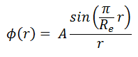
 Let assume a uniform reactor (multiplying system) in the shape of a cylinder of physical radius R and height H. This finite cylindrical reactor is situated in cylindrical geometry at the origin of coordinates. To solve the diffusion equation, we have to replace the Laplacian by its cylindrical form:

Since there is no dependence on angle Θ, we can replace the 3D Laplacian with its two-dimensional form, and we can solve the problem in radial and axial directions. Since the flux is a function of radius – r and height – z only (Φ(r,z)), the diffusion equation can be written as:
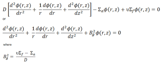
The solution of this diffusion equation is based on the use of the separation-of-variables technique, therefore:
![]()
where R(r) and Z(z) are functions to be determined. Substituting this into the diffusion equation and dividing by R(r)Z(z), we obtain:
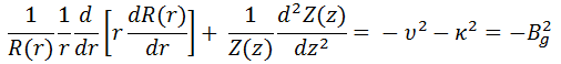
Because the first term depends only on r and the second only on z, both terms must be constants for the equation to have a solution. Suppose we take the constants to be v2 and к2. The sum of these constants must be equal to Bg2 = v2 + к2. Now we can separate variables, and the neutron flux must satisfy the following differential equations:
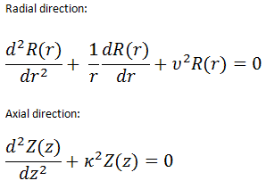
Solution for the radial direction
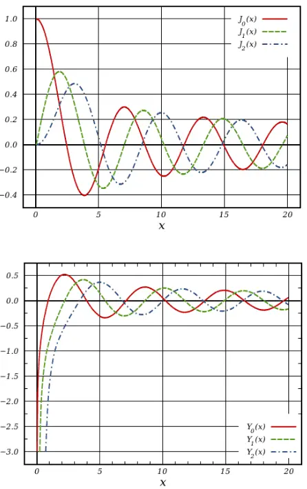 The differential equation for radial direction is called Bessel’s equation, and it is well known to mathematicians. In this case, the Bessel’s equation’s solutions are called the Bessel functions of the first and second kind, Jα(x) and Yα(x), respectively.
For r > 0, this differential equation has two possible solutions, J0(vr) and Y0(vr), the Bessel functions of order zero, which give a general solution:
![]()
From finite flux condition (0≤ Φ(r) < ∞), which required only reasonable values for the flux, it can be derived that C must be equal to zero. The term Y0(vr) goes to -∞ as r ➝0 and therefore cannot be part of a physically acceptable solution. The physically acceptable solution must then be:
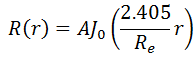
R(r) = AJ0(vr)
The vacuum boundary condition requires the relative neutron flux near the boundary to have a slope of -1/d, i.e., the flux would extrapolate linearly to 0 at a distance d beyond the boundary. This zero flux boundary condition is more straightforward and can be written mathematically as:

If d is not negligible, physical dimensions of the reactor are increased by d, and extrapolated boundary is formulated with dimension Re = R + d, and this condition can be written as Φ(R + d) = Φ(Re) = 0.
Therefore, the solution must be R(Re) = A J0(vRe) = 0. The function of J0(r) has several zeroes. The first is at r1 = 2.405, and the second at r2 = 5.6. However, because the neutron flux cannot have negative values, the only physically acceptable value for v is 2.405/Re. The solution of the diffusion equation is:
Solution for axial direction
The solution for axial direction has been solved in previous sections (Infinite Slab Reactor), and therefore it has the same solution. The solution in an axial direction is:
Solution for radial and axial directions
The full solution for the neutron flux distribution in the finite cylindrical reactor is, therefore:
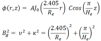
where Bg2 is the total geometrical buckling.
The constants A and C must be added that they cannot be obtained from the diffusion equation because they give the absolute value of neutron flux. The neutron flux can have any value, and the critical reactor can operate at any power level. It should be noted this flux shape is only in a hypothetical case in a uniform homogeneous cylindrical reactor at low power levels (at “zero power criticality”).
In a power reactor core, the neutron flux can reach, for example, about 3.11 x 10¹³ neutrons.cm-2.s-1, but this value depends significantly on many parameters (type of fuel, fuel burnup, fuel enrichment, position in fuel pattern, etc.).
The power level does not influence the criticality (keff) of a power reactor unless thermal reactivity feedbacks act (operation of a power reactor without reactivity feedbacks is between 10E-8% – 1% of rated power).