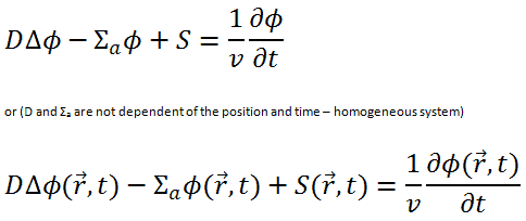
Solutions of the Diffusion Equation – Non-multiplying Systems
in various geometries that satisfy the boundary conditions discussed in the previous section.
We will start with simple systems and increase complexity gradually. The most important assumption is that all neutrons are lumped into a single energy group. They are emitted and diffuse at thermal energy (0.025 eV).
In the first section, we will deal with neutron diffusion in a non-multiplying system, i.e., in a system where fissile isotopes are missing, the fission cross-section is zero. The neutrons are emitted by an external neutron source. We will assume that the system is uniform outside the source, i.e., D and Σa are constants.
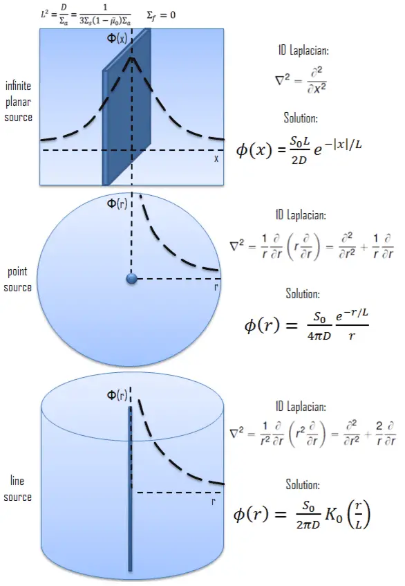
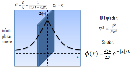 Let assume the neutron source (with strength S0) as an infinite plane source (in y-z plane geometry). In this geometry the flux varies so slowly in y and z allowing us to eliminate the y and z derivatives from ∇2. The flux is then a function of x only, and therefore the Laplacian and diffusion equation (outside the source) can be written as (everywhere except x = 0):

For x > 0, this diffusion equation has two possible solutions exp(x/L) and exp(-x/L), which give a general solution:
Φ(x) = Aexp(x/L) + Cexp(-x/L)
Note that B is not usually used as a constant because B is reserved for a buckling parameter. To determine the coefficients A and C, we must apply boundary conditions.
From finite flux condition (0≤ Φ(x) < ∞), which required only reasonable values for the flux, it can be derived that A must be equal to zero. The term exp(x/L) goes to ∞ as x ➝∞ and therefore cannot be part of a physically acceptable solution for x > 0. The physically acceptable solution for x > 0 must then be:
Φ(x) = Ce-x/L
where C is a constant that can be determined from the source condition at x ➝0.
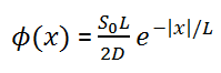
If S0 is the source strength per unit area of the plane, then the number of neutrons crossing outwards per unit area in the positive x-direction must tend to S0 /2 as x ➝0.

So that the solution may be written:
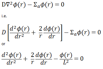
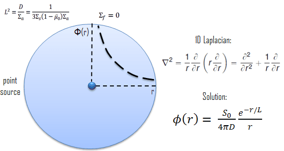 Let assume the neutron source (with strength S0) as an isotropic point source situated in spherical geometry. This point source is placed at the origin of coordinates. To solve the diffusion equation, we have to replace the Laplacian with its spherical form:

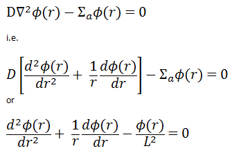
We can replace the 3D Laplacian with its one-dimensional spherical form because there is no dependence on an angle (whether polar or azimuthal). The source is assumed to be an isotropic source (there is the spherical symmetry). The flux is then a function of radius – r only, and therefore the diffusion equation (outside the source) can be written as (everywhere except r = 0):
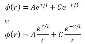
If we make the substitution Φ(r) = 1/r ψ(r), the equation simplifies to:
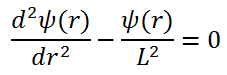
For r > 0, this differential equation has two possible solutions exp(r/L) and exp(-r/L), which give a general solution:
Note that B is not usually used as a constant because B is reserved for a buckling parameter. To determine the coefficients A and C, we must apply boundary conditions.
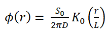
To find constants A and C, we use the identical procedure as in the case of the infinite planar source. From finite flux condition (0≤ Φ(r) < ∞), which required only reasonable values for the flux, it can be derived that A must be equal to zero. The term exp(r/L)/r goes to ∞ as r ➝∞ and therefore cannot be part of a physically acceptable solution for r > 0. The physically acceptable solution for r > 0 must then be:
Φ(r) = Ce-r/L/r
where C is a constant that can be determined from source condition at x ➝0.
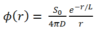
If S0 is the source strength, then the number of neutrons crossing a sphere outwards in the positive r-direction must tend to S0 as r ➝0.
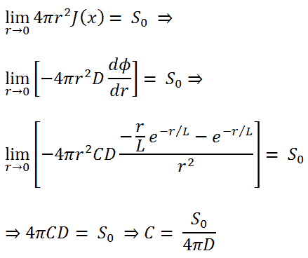
So that the solution may be written:
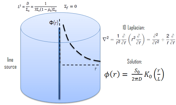 Let assume the neutron source (with strength S0) as an isotropic line source situated in an infinite cylindrical geometry. This line source is placed at r = 0. To solve the diffusion equation, we have to replace the Laplacian by its cylindrical form:
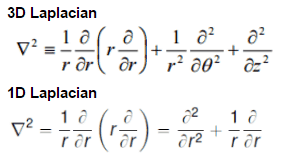
Since there is no dependence on angle Θ and z-coordinate, we can replace the 3D Laplacian with its one-dimensional form and solve the problem only in the radial direction. The source is assumed to be an isotropic source. Since the flux is a function of radius – r only, the diffusion equation (outside the source) can be written as (everywhere except r = 0):
 This differential equation is called Bessel’s equation, and it is well known to mathematicians. In this case, the solutions to the Bessel’s equation are called the modified Bessel functions (or occasionally the hyperbolic Bessel functions) of the first and second kind, Iα(x) and Kα(x), respectively.
For r > 0, this differential equation has two possible solutions, I0(r/L) and K0(r/L), the modified Bessel functions of order zero, which give a general solution:

To find constants A and C, we use the identical procedure as in the case of the infinite planar source. From finite flux condition (0≤ Φ(r) < ∞), which required only reasonable values for the flux, it can be derived that A must be equal to zero. The term I0(r/L) goes to ∞ as r ➝∞ and therefore cannot be part of a physically acceptable solution for r > 0. The physically acceptable solution for r > 0 must then be:
Φ(r) = C.K0(r/L)
where C is a constant that can be determined from the source condition at r ➝0.
If S0 is the source strength, then the number of neutrons crossing a cylinder outwards in the positive r-direction must tend to S0 as r ➝0.
So that the solution may be written:
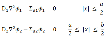
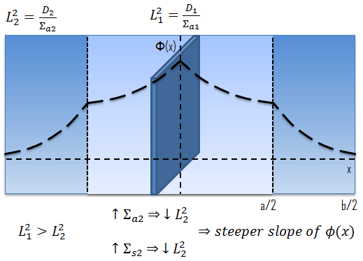
where a is the real width of zone 1 and b is the outer dimension of the diffusion environment, including the extrapolated distance. With problems involving two different diffusion media, the interface boundary conditions play a crucial role and must be satisfied:
At interfaces between two different diffusion media (such as between the reactor core and the neutron reflector), on physical grounds, the neutron flux and the normal component of the neutron current must be continuous. In other words, φ and J are not allowed to show a jump.
1., 2. Interface Conditions
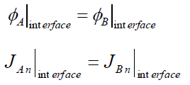
It must be added, as J must be continuous, the flux gradient will show a jump if the diffusion coefficients in both media differ from each other. Since the solution of these two diffusion equations requires four boundary conditions, we have to use two boundary conditions more.
3. Finite Flux Condition
The solution must be finite in those regions where the equation is valid, except perhaps at artificial singular points of a source distribution. This boundary condition can be written mathematically as:
![]() 4. Source Condition
4. Source Condition
The presence of the neutron source can be used as a boundary condition because it is necessary that all neutrons flowing through the bounding area of the source must come from the neutron source. This boundary condition depends on the source geometry, and for planar source can be written mathematically as:
![]()
For x > 0, these diffusion equations have the following appropriate solutions:
Φ1(x) = A1exp(x/L1) + C1exp(-x/L1)
and
Φ2(x) = A2exp(x/L2) + C2exp(-x/L2)
where the four constants must be determined with the use of the four boundary conditions. The typical neutron flux distribution in a simple two-region diffusion problem is shown in the picture below.