If the reactivity is constant, the model of point kinetics equations contains a set (1 + 6) of linear ordinary differential equations with constant coefficient and can be solved analytically. Solution of six-group point kinetics equations with Laplace transformation leads to the relation between the reactivity and the reactor period. This relation is known as the inhour equation (which comes from inverse hour, when it was used as a unit of reactivity that corresponded to e-fold neutron density change during one hour) may be derived.
General Form:
The point kinetics equations may be solved for the case of an initially critical reactor without external source in which the properties are changed at t = 0 in such a way as to introduce a step reactivity ρ0 which is then constant over time. The system of coupled first-order differential equations can be solved with Laplace transformation or by trying the solution n(t) = A.exp(s.t) (equation for the neutron flux) and Ci(t) = Ci,0.exp(s.t) (equations for the density of precursors).
Substitution of these assumed exponential solutions in the equation for precursors gives the relation between the coefficients of the neutron density and the precursors.
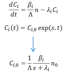
The subsequent substitution in the equation for neutron density yields an equation for s, which after some manipulation can be written as:
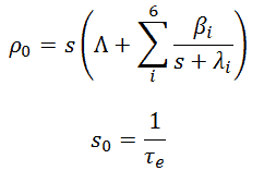

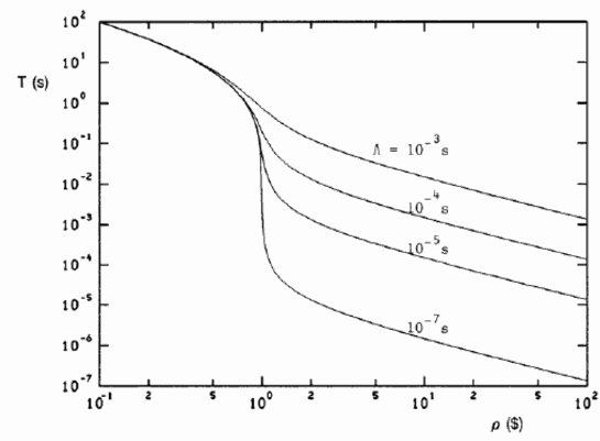
This equation is known as the inhour equation, since the constants of s0 – 6 was originally determined in inverse hours. For a given value of the reactivity ρ the associated values of s0 – 6 are determined with this equation. The following figure shows the relation between ρ and roots s graphically. From this figure it can be seen that for a given value of ρ seven solutions exist for s. The figure indicates that for positive reactivity only s0 is positive. The remaining terms rapidly die away, yielding an asymptotic solution in the form:
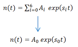
where s0 = 1/τe is the stable reactor period or asymptotic period of reactor. This root, s0, is positive for ρ > 0 and negative for ρ < 0, therefore this root describes the reactor response, which is lasting after the transition phenomena have died out. The figure also shows that a negative reactivity leads to a negative period: All of the si are negative, but the root s0 will die away more slowly than the others. Thus the solution n(t) = A0exp(s0t) is valid for positive as well as negative reactivity insertions.
To determine the reactivity required to produce a given period a plot of ρ vs. τe must be constructed using the delayed neutron data for a particular fissionable isotope or mix of isotopes, and for a given prompt generation time. To determine the stable reactor period, which results from a given reactivity insertion, it is convenient to use the following form of inhour equation.
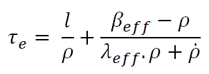
where:
βeff = effective delayed neutron fraction
λeff = effective delayed neutron precursor decay constant
τe = reactor period
ρ = reactivity
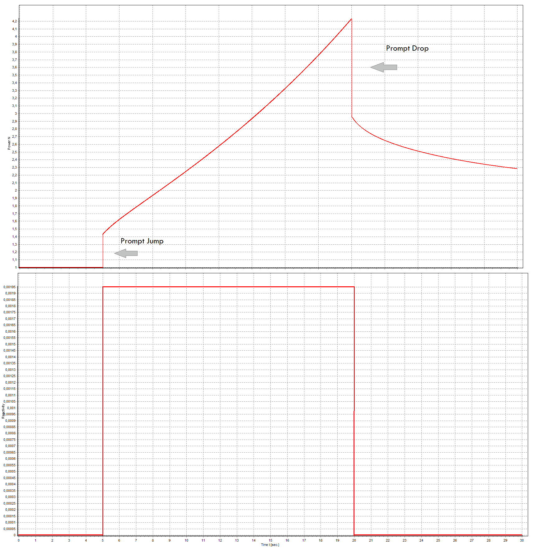
The first term in this formula is the prompt term and it causes that the positive reactivity insertion is followed immediately by a immediate power increase called the prompt jump. This power increase occurs because the rate of production of prompt neutrons changes immediately as the reactivity is inserted. After the prompt jump, the rate of change of power cannot increase any more rapidly than the built-in time delay the precursor half-lives allow. Therefore the second term in this formula is called the delayed term. The presence of delayed neutrons causes the power rise to be controllable and the reactor can be controlled by control rods or another reactivity control mechanism.
The reactor startup rate is defined as the number of factors of ten that power changes in one minute. Therefore the units of SUR are powers of ten per minute, or decades per minute (dpm). The relationship between reactor power and startup rate is given by following equation:
n(t) = n(0).10SUR.t
where:
SUR = reactor startup rate [dpm – decades per minute]
t = time during reactor transient [minute]
The higher the value of SUR, the more rapid the change in reactor power. The startup rate may be positive or negative. If SUR is positive, reactor power is increasing. If SUR is negative, reactor power is decreasing. The relationship between reactor period and startup rate is given by following equations:

Example:
Suppose keff = 1.0005 in a reactor with a generation time ld = 0.01s. For this state calculate the reactor period – τe, doubling time – DT and the startup rate (SUR).
ρ = 1.0005 – 1 / 1.0005 = 50 pcm
τe = ld / k-1 = 0.1 / 0.0005 = 200 s
DT = τe . ln2 = 139 s
SUR = 26.06 / 200 = 0.13 dpm
Special Cases of Inhour Equation
As can be seen, this special case results in the same period as in the case of simple point kinetics equation, which also uses the mean generation time with delayed neutrons (ld):
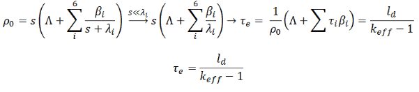
Thus for small reactivities—positive or negative—the reactor period is governed almost completely by the delayed neutron properties. Despite the fact the amount of delayed neutrons is only on the order of tenths of percent of the total amount, the timescale in seconds (τi) plays the extremely important role.
The assumption is s0 ≪ λi. The largest value of τi = 1/λi = 80s, therefore the this formula is valid for periods, τe, higher than 80s. On the other hand, this formula is useful and accurate enough for most purposes for reactivities up to about ρ = 0.0005 = 50pcm.
Note that:
Mean generation time with delayed neutrons (ld):
ld = (1 – β).lp + ∑li . βi => ld = (1 – β).lp + ∑τi . βi
where
- (1 – β) is the fraction of all neutrons emitted as prompt neutrons
- lp is the prompt neutron lifetime
- τi is the mean precursor lifetime, the inverse value of the decay constant τi = 1/λi
- The weighted delayed generation time is given by τ = ∑τi . βi / β = 13.05 s
- Therefore the weighted decay constant λ = 1 / τ ≈ 0.08 s-1
The number, 0.08 s-1, is relatively high and have a dominating effect of reactor time response, although delayed neutrons are a small fraction of all neutrons in the core. This is best illustrated by calculating a weighted mean generation time with delayed neutrons:
ld = (1 – β).lp + ∑τi . βi = (1 – 0.0065). 2 x 10⁻⁵ + 0.085 = 0.00001987 + 0.085 ≈ 0.085
In short, the mean generation time with delayed neutrons is about ~0.1 s, rather than ~10-5 as in section Prompt Neutron Lifetime, where the delayed neutrons were omitted.
Example:
Let us consider that the mean generation time with delayed neutrons is ~0.085 and k (k∞ – neutron multiplication factor) will be step increased by only 0.01% (i.e., 10pcm or ~1.5 cents), that is k∞=1.0000 will increase to k∞=1.0001.
It must be noted such reactivity insertion (10pcm) is very small in case of LWRs (e.g., one step by control rods). The reactivity insertions of the order of one pcm are for LWRs practically unrealizable. In this case the reactor period will be:
T = ld / (k∞-1) = 0.085 / (1.0001-1) = 850s
This is a very long period. In ~14 minutes the neutron flux (and power) in the reactor would increase by a factor of e = 2.718. This is completely different dimension of the response on reactivity insertion in comparison with the case without presence of delayed neutrons, where the reactor period was 1 second.
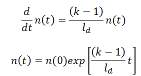
This causes the first root, s0, of the reactivity becomes large compared to each λi. In this case, λi ≪ s0 and therefore, we can ignore the term λi in the denominator of the inhour equation. The inhour equation then takes form:
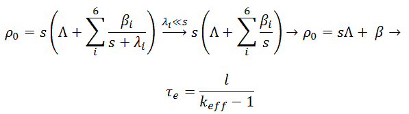
As can be seen, this special case results in the same period as in the case of simple point kinetics equation without delayed neutrons.
Obviously, reaching the reactivity of β (e.g., 650pcm) completely changes the response of a reactor, therefore this situation can only be accidental. As prompt criticality is reached, the distinction between the prompt jump and the reactor period vanishes, for now the prompt neutron lifetime rather than the delayed neutron half-lives largely determines the rate of exponential increase. Reactors with such a kinetics would be very difficult to control by mechanical means such as the movement of control rods. In normal operation, the reactivity of a reactor must remain far below the prompt criticality threshold with sufficient margin.
In design basis accidents (DBA), such a kinetics can occur. For example under RIA conditions (Reactivity-Initiated Accidents) reactors should withstand a jump-like insertion of relatively large (~1 $ or even more) positive reactivity (e.g., in case of control rod ejection) and the PNL (prompt neutron lifetime) plays here the key role. The longer prompt neutron lifetimes can substantially improve kinetic response of reactor (the longer prompt neutron lifetime gives simply slower power increase). Therefore the PNL should be verified in a reload safety evaluation (RSE) process. Management of this accident is based on reactivity feedbacks, especially on the doppler temperature coefficient (DTC). This coefficient is of the highest importance in the reactor stability. The doppler temperature coefficient is generally considered to be even more important than the moderator temperature coefficient (MTC). Especially in case of a control rod ejection the doppler temperature coefficient will be the first and the most important feedback, that will compensate the inserted positive reactivity. The time for heat to be transferred to the moderator is usually measured in seconds, while the fuel temperature coefficient is effective almost instantaneously. Therefore this coefficient is also called the prompt temperature coefficient because it causes an immediate response on changes in fuel temperature.
But even if it were possible to insert an infinite negative reactivity, the neutron flux would not immediately fall to zero. Prompt neutrons will be absorbed almost immediately. It is consistent with the prompt drop formula. Therefore the resulting neutron flux will be:
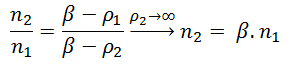
It is obvious, the neutron flux cannot drop below the value βn1. The real values are much higher. The integral worth of all control and emergency rods (PWRs) is for example -9000pcm. It is equal to ρ = -9000/600 = -15β = -0.09 (β= 600pcm = 0.006)
For this negative reactivity the prompt drop is equal to:
n2/n1 = 0.006/(0.006+0.09)=0.063
which is about ten times higher than in case of an infinite negative reactivity insertion.
The neutron flux then continues to fall according to stable period. The first root of reactivity equation occurs at s0 = – λ1. the decay constant of the long-lived precursors group. The shortest negative stable period is then τe = – 1/λ1 = -80s. The neutron flux cannot be reduced more rapidly than this period. On the other hand, the prompt drop causes an immediate drop to about 6% of rated power and within few tens of seconds the thermal power which originates from nuclear fission is below the thermal power which originates from decay heat.