Article Summary & FAQs
What is the Reynolds number?
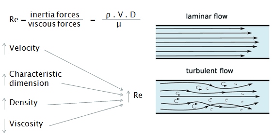
The Reynolds number represents the ratio of inertial forces to viscous forces and is a convenient parameter for predicting if a flow condition will be laminar or turbulent. It is defined as a characteristic length multiplied by a characteristic velocity and divided by the kinematic viscosity.
Key Facts
- Osborn Reynolds discovered that the flow regime depends mainly on the ratio of the inertia forces to viscous forces in the fluid.
- When the viscous forces are dominant (slow flow, low Re), they are sufficient to keep all the fluid particles in line, then the flow is laminar.
- When the inertial forces dominate over the viscous forces (when the fluid flows faster and Re is larger), the flow is turbulent.
- It is defined as:
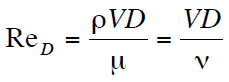 in which V is the mean flow velocity, D is a characteristic linear dimension, ρ fluid density, μ dynamic viscosity, and ν kinematic viscosity.
 - The Reynolds number can be used to compare a real situation (e.g.,, airflow around an airfoil and water flow in a pipe) with a small-scale model.
- Determine the type of flow (internal, external, steady-state, etc.).
- Choose or calculate the characteristic linear dimension
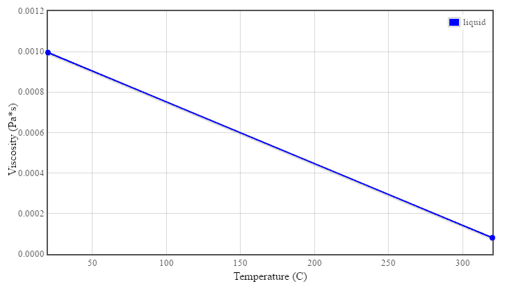
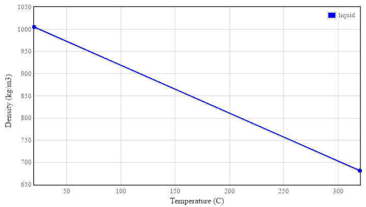
- From tables, determine the viscosity and the density of the fluid.
- Forgiven flow velocity, calculate the Reynolds number.
It is a dimensionless number comprised of the physical characteristics of the flow. An increasing Reynolds number indicates increasing turbulence of flow.
It is defined as:

where:
V is the flow velocity,
D is a characteristic linear dimension, (travelled length of the fluid; hydraulic diameter etc.)
ρ fluid density (kg/m3),
μ dynamic viscosity (Pa.s),
ν kinematic viscosity (m2/s); ν = μ / ρ.

Reynolds Number
The Reynolds number represents the ratio of inertial forces to viscous forces and is a convenient parameter for predicting if a flow condition will be laminar or turbulent. It is defined as a characteristic length multiplied by a characteristic velocity and divided by the kinematic viscosity.
It can be interpreted that when the viscous forces are dominant (slow flow, low Re), they are sufficient enough to keep all the fluid particles in line, then the flow is laminar. Even very low Re indicates viscous creeping motion, where inertia effects are negligible. When the inertial forces dominate over the viscous forces (when the fluid flows faster and Re is larger), the flow is turbulent. The transition from laminar to turbulent flow depends on the surface geometry, surface roughness, free-stream velocity, surface temperature, and type of fluid, among other things.
 It must be noted and the Reynolds number is one of the characteristic numbers (standardized in ISO 80000-11:2019), which can be used to compare a real situation (e.g.,, airflow around an airfoil and water flow in a pipe) with a small-scale model.
The Reynolds number is defined as:
where:
V is the flow velocity,
D is a characteristic linear dimension (traveled length of the fluid; hydraulic diameter etc.)
ρ fluid density (kg/m3),
μ dynamic viscosity (Pa.s),
ν kinematic viscosity (m2/s); ν = μ / ρ.
Application of Reynolds Number
The Reynolds number plays an important part in calculations in fluid dynamics and heat transfer problems.
- It is essential to calculate the friction factor in a few of the equations of fluid mechanics, including the Darcy-Weisbach equation.
- It is essential for heat transfer calculations since many other characteristic numbers (e.g.,, Nusselt number) depend on the flow regime.
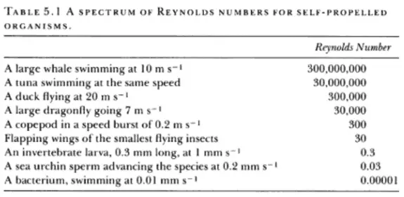
- It is used when modeling the movement of organisms swimming through water.
- It is used to predict the transition from laminar to turbulent flow and is used to scale similar but different-sized flow situations, such as between an aircraft model in a wind tunnel and the full-size version.
- The predictions of the onset of turbulence and the ability to calculate scaling effects can be used to help predict fluid behavior on a larger scale, such as in local or global air or water movement and thereby the associated meteorological and climatological effects.
History of Reynolds Number
The concept was introduced by George Stokes in 1851, but Arnold Sommerfeld named the Reynolds number in 1908 after Osborne Reynolds (1842–1912), who performed exhaustive experiments in the 1880s. Osborn Reynolds discovered that the flow regime depends mainly on the ratio of the inertia forces to viscous forces in the fluid.
This study is closely associated with the boundary layer concept. The study of flows developing along a solid boundary is of primary importance for many engineering problems, such as the drag reduction of airplane wings in the aeronautics field. In the boundary layer concept, introduced by Prandtl (1904), the field of wall-bounded flows can be divided into two regions:
- a thin region near the wall called the boundary layer, where strong velocity gradients occur, inducing large viscous shearing forces that must be taken into account and
- a region outside the boundary layer, where the friction forces can be neglected, and where, therefore, inviscid fluid theory offers a good approximation.
The major contribution of the boundary layer concept was to overcome the D’Alembert paradox and to reunify theoretical hydrodynamics (derived in the framework of the perfect fluid hypothesis) with empirical laws from hydraulics. Fundamental research on boundary layers focuses on studying canonical configurations such as pipe flow, channel flow, or flow over a flat plate.
For the flow over a flat plate, it can be seen, near the leading edge of the plate, the régime of the boundary layer is laminar: the flow is two-dimensional and steady. As the boundary layer develops, the flow becomes critical and undergoes the transition from the laminar to the turbulent regime: instabilities appear and propagate, giving birth to turbulent spots, irregularly distributed in space and time. As the distance x from the leading edge increases (i.e., as the Reynolds Number increases), the flow becomes unstable, and finally, for higher Reynolds numbers, the boundary layer is turbulent, and the streamwise velocity is characterized by unsteady (changing with time) swirling flows inside the boundary layer. Turbulence always occurs at large Reynolds numbers.
Critical Reynolds Number
The Reynolds number at which the flow becomes turbulent is called the critical Reynolds number. The value of the critical Reynolds number is different for different geometries.
- For flow over a flat plate, the generally accepted value of the critical Reynolds number is Rex ~ 500000.
- For flow in a pipe of diameter D, experimental observations show that for “fully developed” flow, laminar flow occurs when ReD < 2300, and turbulent flow occurs when ReD > 3500.
- For a sphere in a fluid, the characteristic length-scale is the sphere’s diameter, and the characteristic velocity is that of the sphere relative to the fluid. Purely laminar flow only exists up to Re = 10 under this definition.
Reynolds’ law of similarity
For two flows to be similar, they must have the same geometry and equal Reynolds and Euler numbers. When comparing fluid behavior at corresponding points in a model and a full-scale flow, the following holds:
Remodel = Re
Eumodel = Eu
For example, let us compare Reynolds numbers of an actual vehicle and a half-scale model as shown in the following diagram. The Reynolds numbers of both agree when the velocity of the half-scale model is doubled. In this state, the proportions of both cases’ viscous force and inertia forces are equal; hence, the surrounding flows can be defined as similar.
This allows engineers to perform experiments with reduced scale models in water channels or wind tunnels and correlate the data to the actual flows, saving costs during experimentation and lab time. True dynamic similitude may require matching other dimensionless numbers, such as the Mach number used in compressible flows or the Froude number that governs open-channel flows.
Laminar vs. Turbulent Flow
Laminar flow:
- Re < 2000
- ‘low’ velocity
- Fluid particles move in straight lines
- Layers of water flow over one another at different speeds with virtually no mixing between layers.
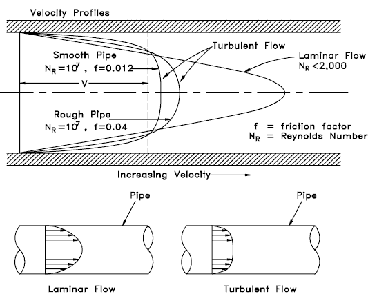
- The flow velocity profile for laminar flow in circular pipes is parabolic in shape, with a maximum flow at the center of the pipe and a minimum flow at the pipe walls.
- The average flow velocity is approximately one-half of the maximum velocity.
- Simple mathematical analysis is possible.
- Rare in practice in water systems.
Turbulent Flow:
- Re > 4000
- ‘high’ velocity
- The flow is characterized by the irregular movement of particles of the fluid.
- Average motion is in the direction of the flow.
- The flow velocity profile for turbulent flow is fairly flat across the center section of a pipe and drops rapidly extremely close to the walls.
- The average flow velocity is approximately equal to the velocity at the center of the pipe.
- Mathematical analysis is very difficult.
- The most common type of flow.
All fluid flow is classified into one of two broad categories or regimes. These two flow regimes are:
- Single-phase Fluid Flow
- Multi-phase Fluid Flow (or Two-phase Fluid Flow)
This is a basic classification. All of the fluid flow equations (e.g.,, Bernoulli’s Equation) and relationships discussed in this section (Fluid Dynamics) were derived for the flow of a single phase of fluid, whether liquid or vapor. Solution of multi-phase fluid flow is very complex and difficult, and therefore it is usually in advanced courses of fluid dynamics.
 Another usually more common classification of flow regimes is according to the shape and type of streamlines. All fluid flow is classified into one of two broad categories. The fluid flow can be either laminar or turbulent, and therefore these two categories are:
- Laminar Flow
- Turbulent Flow
Laminar flow is characterized by smooth or regular paths of particles of the fluid. Therefore the laminar flow is also referred to as streamline or viscous flow. In contrast to laminar flow, turbulent flow is characterized by the irregular movement of particles of the fluid. The turbulent fluid does not flow in parallel layers, the lateral mixing is very high, and there is a disruption between the layers. Most industrial flows, especially those in nuclear engineering, are turbulent.
The flow regime can also be classified according to the geometry of a conduit or flow area. From this point of view, we distinguish:
- Internal Flow
- External Flow
Internal flow is a flow for which a surface confines the fluid. Detailed knowledge of the behavior of internal flow regimes is important in engineering because circular pipes can withstand high pressures and hence are used to convey liquids. On the other hand, external flow flows in which boundary layers develop freely, without constraints imposed by adjacent surfaces. Detailed knowledge of the behavior of external flow regimes is of importance, especially in aeronautics and aerodynamics.
Reynolds Number Regimes
Laminar flow. For practical purposes, if the Reynolds number is less than 2000, the flow is laminar. The accepted transition Reynolds number for flow in a circular pipe is Red,crit = 2300.
Transitional flow. At Reynolds numbers between about 2000 and 4000, the flow is unstable due to the onset of turbulence. These flows are sometimes referred to as transitional flows.
Turbulent flow. If the Reynolds number is greater than 3500, the flow is turbulent. Most fluid systems in nuclear facilities operate with turbulent flow.
Reynolds Number and Internal Flow
The configuration of the internal flow (e.g.,, flow in a pipe) is a convenient geometry for heating and cooling fluids used in energy conversion technologies such as nuclear power plants.
In general, this flow regime is important in engineering because circular pipes can withstand high pressures and hence are used to convey liquids. Non-circular ducts are used to transport low-pressure gases, such as air in cooling and heating systems.
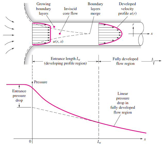
For the internal flow regime, an entrance region is typical. In this region, a nearly inviscid upstream flow converges and enters the tube. The hydrodynamic entrance length is introduced to characterize this region and is approximately equal to:
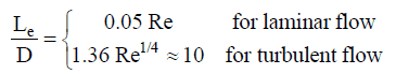
The maximum hydrodynamic entrance length, at ReD,crit = 2300 (laminar flow), is Le = 138d, where D is the diameter of the pipe. This is the longest development length possible. In turbulent flow, the boundary layers grow faster, and Le is relatively shorter. For any given problem, Le / D has to be checked to see if Le is negligible compared to the pipe length. At a finite distance from the entrance, the entrance effects may be neglected because the boundary layers merge and the inviscid core disappears. The tube flow is then fully developed.
Power-law velocity profile – Turbulent velocity profile
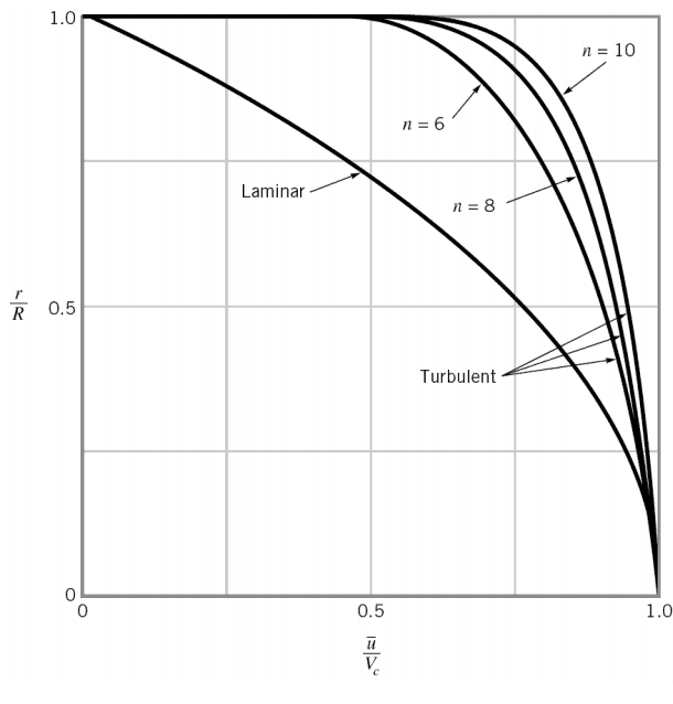
 The velocity profile in turbulent flow is flatter in the central part of the pipe (i.e., in the turbulent core) than in laminar flow. The flow velocity drops rapidly, extremely close to the walls. This is due to the diffusivity of the turbulent flow.
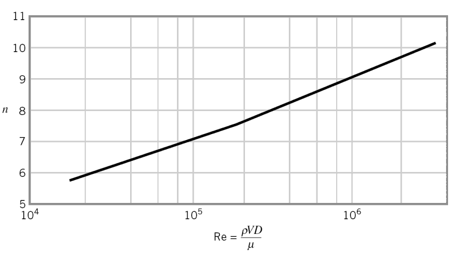
In the case of turbulent pipe flow, there are many empirical velocity profiles. The simplest and the best known is the power-law velocity profile:
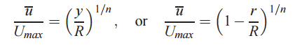
where the exponent n is a constant whose value depends on the Reynolds number. This dependency is empirical, and it is shown in the picture. In short, the value n increases with increasing Reynolds number. The one-seventh power-law velocity profile approximates many industrial flows.
Hydraulic Diameter
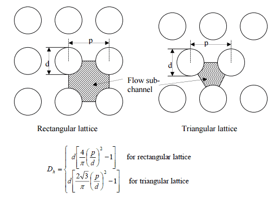
Since the characteristic dimension of a circular pipe is an ordinary diameter D and especially reactors contain non-circular channels, the characteristic dimension must be generalized.
For these purposes, the Reynolds number is defined as:
where Dh is the hydraulic diameter:

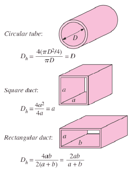 The hydraulic diameter, Dh, is a commonly used term when handling flow in non-circular tubes and channels. The hydraulic diameter transforms non-circular ducts into pipes of equivalent diameter. Using this term, one can calculate many things in the same way as for a round tube. In this equation, A is the cross-sectional area, and P is the wetted perimeter of the cross-section. The wetted perimeter for a channel is the total perimeter of all channel walls that contact the flow.
Example: Reynolds number for primary piping and a fuel bundle
It is an illustrative example, following data do not correspond to any reactor design.
Pressurized water reactors are cooled and moderated by high-pressure liquid water (e.g.,, 16MPa). At this pressure, water boils at approximately 350°C (662°F). The inlet temperature of the water is about 290°C (⍴ ~ 720 kg/m3). The water (coolant) is heated in the reactor core to approximately 325°C (⍴ ~ 654 kg/m3) as the water flows through the core.
The primary circuit of typical PWRs is divided into 4 independent loops (piping diameter ~ 700mm). Each loop comprises a steam generator and one main coolant pump. Inside the reactor pressure vessel (RPV), the coolant first flows down outside the reactor core (through the downcomer). The flow is reversed up through the core from the bottom of the pressure vessel, where the coolant temperature increases as it passes through the fuel rods and the assemblies formed by them.
Assume:
- the primary piping flow velocity is constant and equal to 17 m/s,
- the core flow velocity is constant and equal to 5 m/s,
- the hydraulic diameter of the fuel channel, Dh, is equal to 1 cm
- the kinematic viscosity of the water at 290°C is equal to 0.12 x 10⁻⁶ m2/s
See also: Example: Flow rate through a reactor core
Determine
- the flow regime and the Reynolds number inside the fuel channel
- the flow regime and the Reynolds number inside the primary piping
The Reynolds number inside the primary piping is equal to:
ReD = 17 [m/s] x 0.7 [m] / 0.12×10⁻⁶ [m2/s] = 99 000 000
This fully satisfies the turbulent conditions.
The Reynolds number inside the fuel channel is equal to:
ReDH = 5 [m/s] x 0.01 [m] / 0.12×10⁻⁶ [m2/s] = 416 600
This also fully satisfies the turbulent conditions.
Reynolds Number and External Flow
The Reynolds number describes the external flow naturally as well. In general, when a fluid flows over a stationary surface, e.g.,, the flat plate, the bed of a river, or the pipe wall, the fluid touching the surface is brought to rest by the shear stress at the wall. The boundary layer is the region in which flow adjusts from zero velocity at the wall to a maximum in the mainstream of the flow.
Basic characteristics of all laminar and turbulent boundary layers are shown in the developing flow over a flat plate. The stages of the formation of the boundary layer are shown in the figure below:
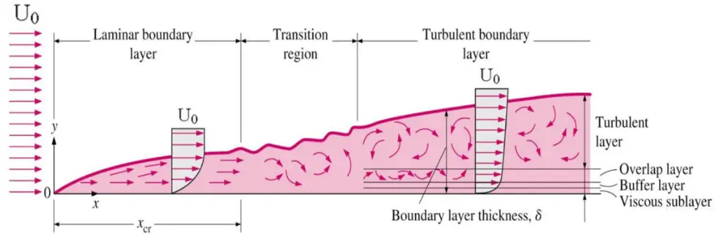
Boundary layers may be either laminar or turbulent, depending on the value of the Reynolds number.
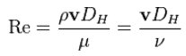
Also, here the Reynolds number represents the ratio of inertia forces to viscous forces and is a convenient parameter for predicting if a flow condition will be laminar or turbulent. It is defined as:
in which V is the mean flow velocity, D is a characteristic linear dimension, ρ fluid density, μ dynamic viscosity, and ν kinematic viscosity.
The boundary layer is laminar for lower Reynolds numbers, and the streamwise velocity uniformly changes as one moves away from the wall, as shown on the left side of the figure. As the Reynolds number increases (with x), the flow becomes unstable. Finally, the boundary layer is turbulent for higher Reynolds numbers, and the streamwise velocity is characterized by unsteady (changing with time) swirling flows inside the boundary layer.
The transition from laminar to turbulent boundary layer occurs when Reynolds number at x exceeds Rex ~ 500,000. The transition may occur earlier, but it is dependent especially on the surface roughness. The turbulent boundary layer thickens more rapidly than the laminar boundary layer due to increased shear stress at the body surface.
The external flow reacts to the edge of the boundary layer just as it would to the physical surface of an object. So the boundary layer gives any object an “effective” shape which is usually slightly different from the physical shape. We define the thickness of the boundary layer as the distance from the wall to the point where the velocity is 99% of the “free stream” velocity.
The boundary layer may lift off or “separate” from the body and create an effective shape much different from the physical shape to make things more confusing. This happens because the flow in the boundary has very low energy (relative to the free stream) and is more easily driven by changes in pressure.
See also: Boundary layer thickness.
See also: Tube in crossflow – external flow.
Special reference: Schlichting Herrmann, Gersten Klaus. Boundary-Layer Theory, Springer-Verlag Berlin Heidelberg, 2000, ISBN: 978-3-540-66270-9