Atkinson Cycle – Atkinson Engine

In 1882, a British engineer, James Atkinson, advanced the study of heat engines by inventing several heat engines that increased efficiency over the Otto cycle. This was achieved by the use of variable engine strokes from a complex crankshaft. The Atkinson cycle is designed to provide higher efficiency at the expense of power density. For two engines of equal displacement volume, an Otto cycle would produce a greater network and greater power if the engines run at the same speed. On the other hand, the Atkinson cycle would have greater thermal efficiency, thus lower fuel consumption.

The first implementation of the Atkinson cycle was in 1882. This engine is known as the “Differential 1882”. It was arranged as an opposed-piston engine, the Atkinson differential engine. The next engine designed by Atkinson in 1887 was named the “Cycle Engine” (see figure)

Recently, it is one of the thermodynamic cycles found in automobile engines and describes the functioning of a spark ignition piston engine. The term Atkinson cycle has been used to describe a modified Otto-cycle engine. The intake valve is held open longer than normal to allow a reverse flow of intake air into the intake manifold. This reduces the compression ratio, but the expansion ratio remains the same. From a mechanical point of view, the Atkinson engine is similar to the Otto engine. The main difference is in camshaft or camshafts.

Atkinson Cycle – Processes

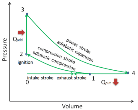
In an Atkinson cycle (modified Otto cycle), the system executing the cycle undergoes a series of four processes: two isentropic (reversible adiabatic) processes alternated with one isochoric process and one isobaric process:

• Isentropic compression (compression stroke) – The gas (fuel-air mixture) is compressed adiabatically from state 1 to state 2, as the piston moves from intake valve closing point (1) to top dead center. The surroundings do work on the gas, increasing its internal energy (temperature) and compressing it. On the other hand, the entropy remains unchanged. The changes in volumes and their ratio (V₁ / V₂) are known as the compression ratio. The compression ratio is smaller than the expansion ratio.
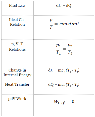
• Isochoric compression (ignition phase) – In this phase (between state 2 and state 3), there is a constant volume (the piston is at rest ) heat transfer to the air from an external source while the piston is at rest at the top dead center. This process is similar to the isochoric process in the Otto cycle. It is intended to represent the ignition of the fuel-air mixture injected into the chamber and the subsequent rapid burning. The pressure rises, and the ratio (P₃ / P₂) is known as the “explosion ratio”.
• Isentropic expansion (power stroke) – The gas expands adiabatically from state 3 to state 4 as the piston moves from top dead center to bottom dead center. The gas works on the surroundings (piston) and loses an amount of internal energy equal to the work that leaves the system. Again the entropy remains unchanged. The volume ratio (V₄ / V₃) is known as the isentropic expansion ratio.
• Isobaric exhaust (exhaust stroke) – The main goal of the modern Atkinson cycle is to allow the pressure in the combustion chamber at the end of the power stroke to be equal to atmospheric pressure. Since there can be atmospheric pressure in the chamber, there is no decompression as in an Otto cycle. The piston moves from the bottom dead center (BDC) to the top dead center (TDC), and the cycle passes points 4 → 1 → 0. The exhaust valve is open in this stroke while the piston pulls exhaust gases out of the chamber.

During the Atkinson cycle, work is done on the gas by the piston between states 1 and 2 (isentropic compression). The gas does work on the piston between stages 3 and 4 (isentropic expansion). The difference between the work done by the gas and the work done on the gas is the network produced by the cycle, and it corresponds to the area enclosed by the cycle curve. The work produced by the cycle times the rate of the cycle (cycles per second) is equal to the power produced by the Atkinson engine.

Isentropic Process

An isentropic process is a thermodynamic process in which the entropy of the fluid or gas remains constant. It means the isentropic process is a special case of an adiabatic process in which there is no transfer of heat or matter. It is a reversible adiabatic process. The assumption of no heat transfer is very important since we can use the adiabatic approximation only in very rapid processes.

Isentropic Process and the First Law

For a closed system, we can write the first law of thermodynamics in terms of enthalpy:

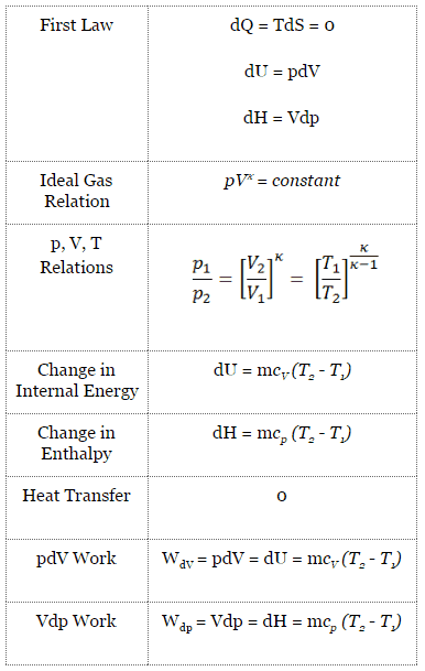
dH = dQ + Vdp

or

dH = TdS + Vdp

Isentropic process (dQ = 0):

dH = Vdp     →     W = H₂ – H₁     →     H₂ – H₁ = C_p (T₂ – T₁)    (for ideal gas)

Isentropic Process of the Ideal Gas

The isentropic process (a special case of the adiabatic process) can be expressed with the ideal gas law as:

pV^κ = constant

or

p₁V₁^κ = p₂V₂^κ

in which κ = c_p/c_v is the ratio of the specific heats (or heat capacities) for the gas. One for constant pressure (c_p) and one for constant volume (c_v). Note that, this ratio κ  = c_p/c_v is a factor in determining the speed of sound in a gas and other adiabatic processes.

Isochoric Process

An isochoric process is a thermodynamic process in which the volume of the closed system remains constant (V = const). It describes the behavior of gas inside the container that cannot be deformed. Since the volume remains constant, the heat transfer into or out of the system does not the p∆V work but only changes the system’s internal energy (the temperature).

Isochoric Process and the First Law

The classical form of the first law of thermodynamics is the following equation:

dU = dQ – dW

In this equation, dW is equal to dW = pdV and is known as the boundary work. Then:

dU = dQ  – pdV

An isochoric process and the ideal gas, all of the heat added to the system, will increase the internal energy.

Isochoric process (pdV = 0):

dU = dQ    (for ideal gas)

dU = 0 = Q – W    →     W = Q      (for ideal gas)

Isochoric Process of the Ideal Gas

The isochoric process can be expressed with the ideal gas law as:

or

On a p-V diagram, the process occurs along a horizontal line with the equation V = constant.

See also: Guy-Lussac’s Law.

Isobaric Process

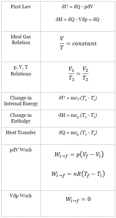
An isobaric process is a thermodynamic process in which the system’s pressure remains constant (p = const). The heat transfer into or out of the system does work and changes the system’s internal energy.

Since there are changes in internal energy (dU) and changes in system volume (∆V), engineers often use the enthalpy of the system, which is defined as:

H = U + pV

Isobaric Process and the First Law

The classical form of the first law of thermodynamics is the following equation:

dU = dQ – dW

In this equation, dW is equal to dW = pdV and is known as the boundary work. In an isobaric process and the ideal gas, part of the heat added to the system will be used to do work, and part of the heat added will increase the internal energy (increase the temperature). Therefore it is convenient to use enthalpy instead of internal energy.

Isobaric process (Vdp = 0):

dH = dQ → Q = H₂ – H₁

At constant entropy, i.e., in the isentropic process, the enthalpy change equals the flow process work done on or by the system.

Isobaric Process of the Ideal Gas

The isobaric process can be expressed with the ideal gas law as:

or

On a p-V diagram, the process occurs along a horizontal line (called an isobar) with the equation p = constant.

See also: Charles’s Law.

Thermal Efficiency for Atkinson Cycle

In general, the thermal efficiency, η_th, of any heat engine is defined as the ratio of the work it does, W, to the heat input at the high temperature, Q_H.

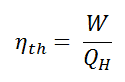
The thermal efficiency, η_th, represents the fraction of heat, Q_H, converted to work. Since energy is conserved according to the first law of thermodynamics and energy cannot be converted to work completely, the heat input, Q_H, must equal the work done, W, plus the heat that must be dissipated as waste heat Q_C into the environment. Therefore we can rewrite the formula for thermal efficiency as:

The heat absorbed occurs during combustion of fuel-air mixture, when the spark occurs, roughly at constant volume. Since there is no work done by or on the system during an isochoric process, the first law of thermodynamics dictates ∆U = ∆Q.

Therefore the heat added and rejected are given by:

Q_add = mc_v (T₃ – T₂)

Q_out = mc_p (T₄ – T₁)

Substituting these expressions for the heat added and rejected in the expression for thermal efficiency yields:

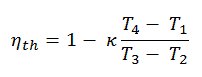
Furthermore, it can be derived that in terms of:

• the ratio V₁/V₂, which is known as the compression ratio – CR
• the ratio V₄/V₃, which is known as the expansion ratio – ER.
• κ = c_p/c_v

The expression for thermal efficiency using these characteristics is:

See above:

Thermodynamic Cycles